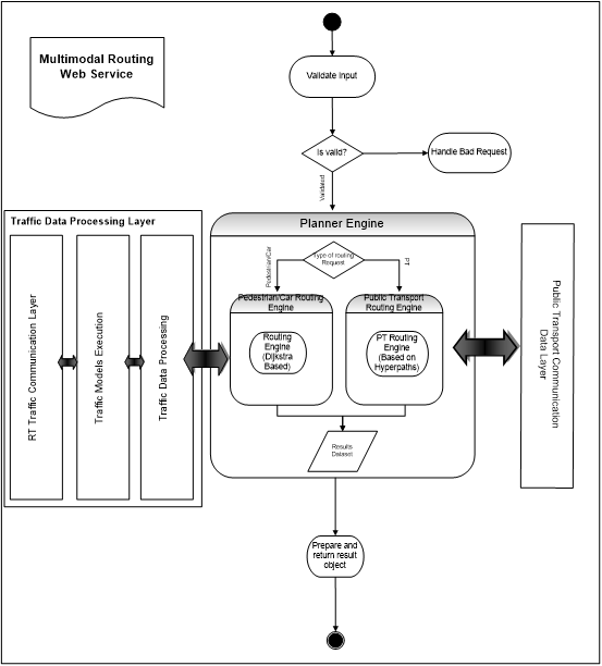
A web service has been developed by CERTH-HIT, which acts as a “wrapper” by utilizing two routing engines, namely the “Car/Pedestrian Routing Engine” and the “Public Transport Routing Engine”. The service provides optimal multimodal routes. The service can be used by any third party, provided that the consumer application (client) is in compliance with the predefined protocols that govern the definition of a web service (SOAP, WSDL, UDDI). The consumption process of the service is independent of the development platform that the third party client uses.
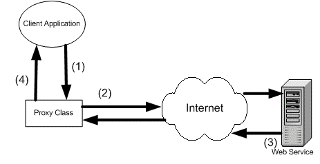
The basic Web service architecture defines the interaction between software clients and the web service as an exchange of messages between them. A Client Application is a piece of software that request the execution of the routing service. The Web Service is the software that responds to that request and returns the result to the client.
The following figure illustrates the procedure that takes place whenever a client performs a route request:
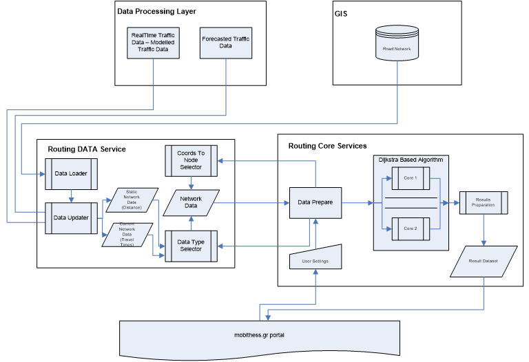
The in-house developed car and pedestrian routing algorithm is based on Dijkstra’s algorithm and provides suggestions to the users about the optimal route they should follow in order to travel by car or on foot from an origin to a destination point. More specifically, the users provide a departure and a destination point and, optionally, one or more intermediate points on a route. Additionally the users, based on their preferences and needs, can choose between the following criteria:
The integrated Car and Pedestrian Routing Engine also provides the following:
The following figure illustrates the procedure that takes place whenever a client performs a route request:
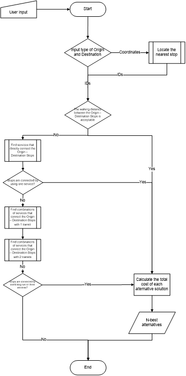
The problem of calculating the optimal combination of routes to plan an urban/interurban journey is one of the most common and interesting problems in the field of transportation and operations research. Planning depends on the specifications of the reference public transport network and its complexity on the one hand and on the unique requirements of individuals on the other hand. In this context, an journey planning algorithm for urban trips that follows the principles of frequency based approach of path choice modeling has been developed. Later on, the algorithm was technically updated to be capable to handle also on interurban network data and environments. Finally, if there is real-time information about the location of the buses and travel times along the bus network, these can be used in order to provide more accurate results.
The PT Routing Engine algorithm has been developed in-house in T-SQL (Microsoft SQL Server 2008+ with spatial support). The algorithmic procedure consists of the following 4 high-level stages:
The main drawback of the Public Transport Routing Engine is that it is limited by design to search for a solution consisting of up to two transits. This happens because the search space of the problem increases rapidly above this number. This may not be a real problem for small to medium size public transport networks such as the public network of Thessaloniki, as –almost- any randomly picked stop can be connected with up to two transits with any other stop in the network. It may though become a problem as the size of the public transport network increases. In such case, some workarounds could be used.
For example the algorithm could split behind the scenes the initial request into smaller sequential sub-requests, by considering the major transit hubs (Bus/Train stations) that exist in the public transport network and by forcing the usage of those hubs as intermediate transit points between the sub-requests. Another workaround could be the increase of the allowed walking distance. In such case, the chances for the algorithm to find a feasible solution increases significantly. In any case, it should be clear that in such case the response time of the algorithm implementation increases further, as well as that the resulting set of solutions may not be the optimal one.
The runtime performance of the algorithm depends heavily on the following parameters (in order of importance):
Network: Public Transport Network of the city of Thessaloniki
The benchmarks of the current implementation of the algorithm on the public transport network with the above characteristics show that the response time of the algorithm manages to be kept in acceptable values in the overwhelming majority of the use cases.
LOGIMATIC addresses container handling automation in terminals through a GIS-based control module compatible with existing Terminal Operating Systems (TOS) for optimized global (yard level) route planning and secure fleet management of Automated Straddle Carriers (ASCs).
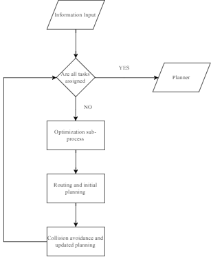
The developed algorithm is a two-stage process:
1) The first stage of the algorithm is focused on assigning tasks to be completed (i.e. containers to be moved) by available ASCs, while subjected to several constraints. It consists of calculating the shortest path between every ASC location and every task location (origin and destination of container movement within the terminal) using the Dijkstra algorithm. Furthermore, it solves a minimization problem in order to assign available ASCs to jobs, minimizing the total distance.
2) The second stage of the algorithm ensures that no collisions occur while the ASCs move within the yard. To do so, it checks for potential collision points and modifies either the speed profile of the straddle carriers, or the routes or the assignments.
The figure illustrates the basic blocks of the algorithm.
The algorithm is not static. To take into account the input of real-time data by a port’s operating system, the algorithm is continuously updated and re-calculated. The real-time data are the actual positions of the Automated Straddle Carriers and the timestamps of those positions in the port yard, which the algorithm uses to compare if the planning output matches the actual movement of the ASCs and if not it re-calculates assignments, trajectories and speeds.
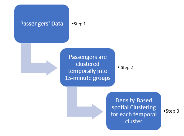
The module aggregates round-trip requests by passengers and produces clusters that can be served by one taxi.
The algorithm that was developed is based on the density-based approach.
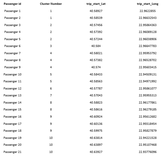
It uses data collected from the potential passengers. At the end of each day, the passengers declare their points of origin, time of departure, points of destination (and similarly for the return trip). The data are used to calculate which passengers could be grouped together and share a taxi from their origin to their destination. The figure below illustrates the process of the clustering algorithm.
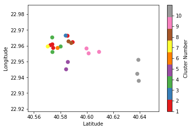
For example, 20 passengers are clustered for one route as follows:
The main scope is the development of an algorithm that will predict the traffic status in the city of Thessaloniki. This approach integrates machine learning techniques using traffic counts and speeds as well as the skewness, kurtosis and standard deviation of the speed, to train an appropriate Neural Network Model for efficient and robust traffic speed prediction. The considerable amount and the nature of the data and the advantage of multiple learning algorithms led us to use Artificial Neural Networks. We want to detect all possible interactions and complex nonlinear or linear relationships, to provide better speed predictions.
For this work, in strong collaboration with Open Knowledge Foundation Greece (okfg) have created a package (TrafficBDE ) in R Software, available on Github. The user selects the road and the date time to predict the wanted variable, either the mean speed or the entries, for this road at this date time and also how many steps forward they want the predicted value to cover.
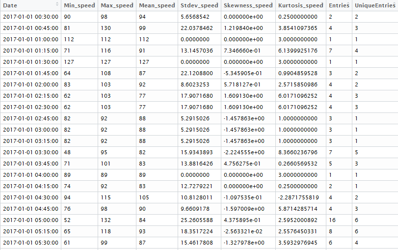
Apart from the input data, there are some features that are being used to train a more accurate model. These features are statistical measures of the mean speed of each Link id in a particular quarter. Namely, these measures refer to standard deviation, skewness and kurtosis.
Firstly, the algorithm filters the historical data of the roads based on the Link id and direction selected by the user, and then the algorithm keeps the data of the previous two weeks from the date time wanted and calculates the features, mentioned above, of the speed. Afterwards, the algorithm checks if all the quarters exist, this means 1344 quarters for two weeks. If there are missing quarters, they are created, and linear interpolation fills the rest data values. When the data are completed, they are split into the train set and test set, and they are processed and normalized between 0 and 1.
Due to its simplicity and the performance of nonlinear patterns, the model used in this algorithm is Multilayer perceptron (MLP). The algorithm decides which Neural Network model will be able to provide the most accurate prediction, performing 10-fold cross validation in the hidden layers to detect the combination of layers and nodes with the minimum average error, where the dataset is being split into ten independent subsets, ten times. Each time a different subset is held out and is used as the test set, while the rest 9 (k-1) subsets form the train set. Finally, after having chosen the best model, the algorithm provides the predicted value.
The input data of the model
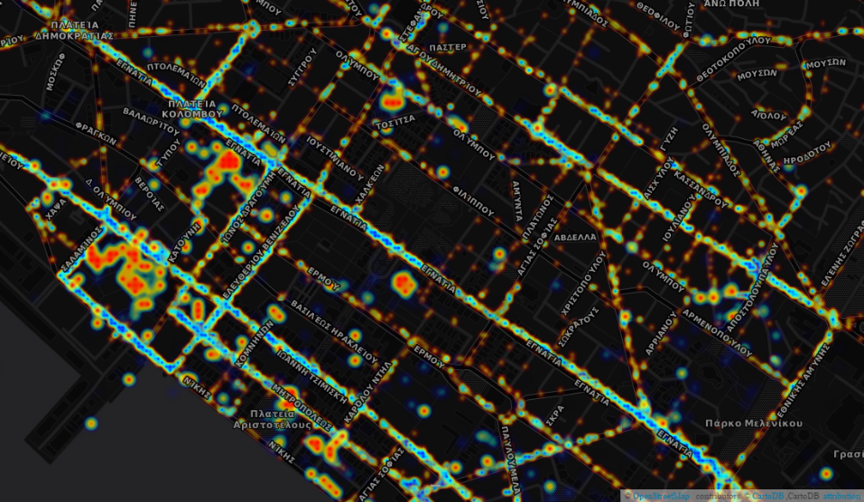
The above methodology is applied to the FCD collected in Thessaloniki, which is generated by 1200 taxi vehicles circulating in average between 16 and 24 hours per day, which periodically (each 6-10 seconds) send pulses containing their location and speed. The total amount of data collected and processed reaches 2,500 pulses per minute, with daily totals at approximately 1.5 million.
Specifically, the data consist of traffic counts and speeds. Roads are divided into parts based on the length and location, and each part has a Link id. Also, depending on the direction of the road, the value 1 or 2 is assigned to it. The date time refers to a specific quarter of the time when the measurements were made. The entries show how many GPS were spotted, and the unique entries refer to the different GPS located on each road at the particular time.
The available data are the historical data of three random roads with links for January in 2017. The features mentioned were calculated and algorithm chose the Neural Network model based on 10-fold cross validation.
We perform two types of test. The first one shows the results of the prediction of eight sequentially date times. As the second type provides the prediction 4 steps forward of the date time, i.e. in the first step, the algorithm uses the historical data to predict the speed value of the first quarter. The predicted value will be used in the second step to predict the speed value of the next quarter. The same process continues until we reach the last quarter.
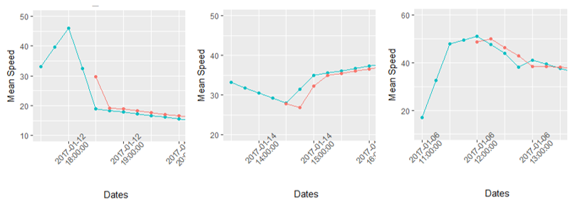
The following figures are the results of the first test. In all three figures, the predicted values follow the pattern. It is worth noting that in cases where the pattern changed abruptly, giving a slightly increased Root Mean Square (RMSE) but still not higher than 10.5km/h and less than 6.5km/h in the three selected links, the algorithm recognised the changed pattern and followed it in the next predictions.
Plot with the Real (blue) and the Predicted (red) values
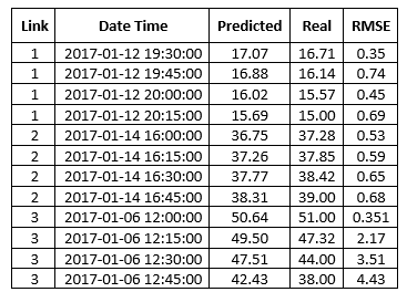
Table 2 shows the results of the 4-step forward case. Taking a look at the results, we can see the prediction value does not differ from the real, and the algorithm captures the changes in mean speed.
Results of the prediction in the three selected links
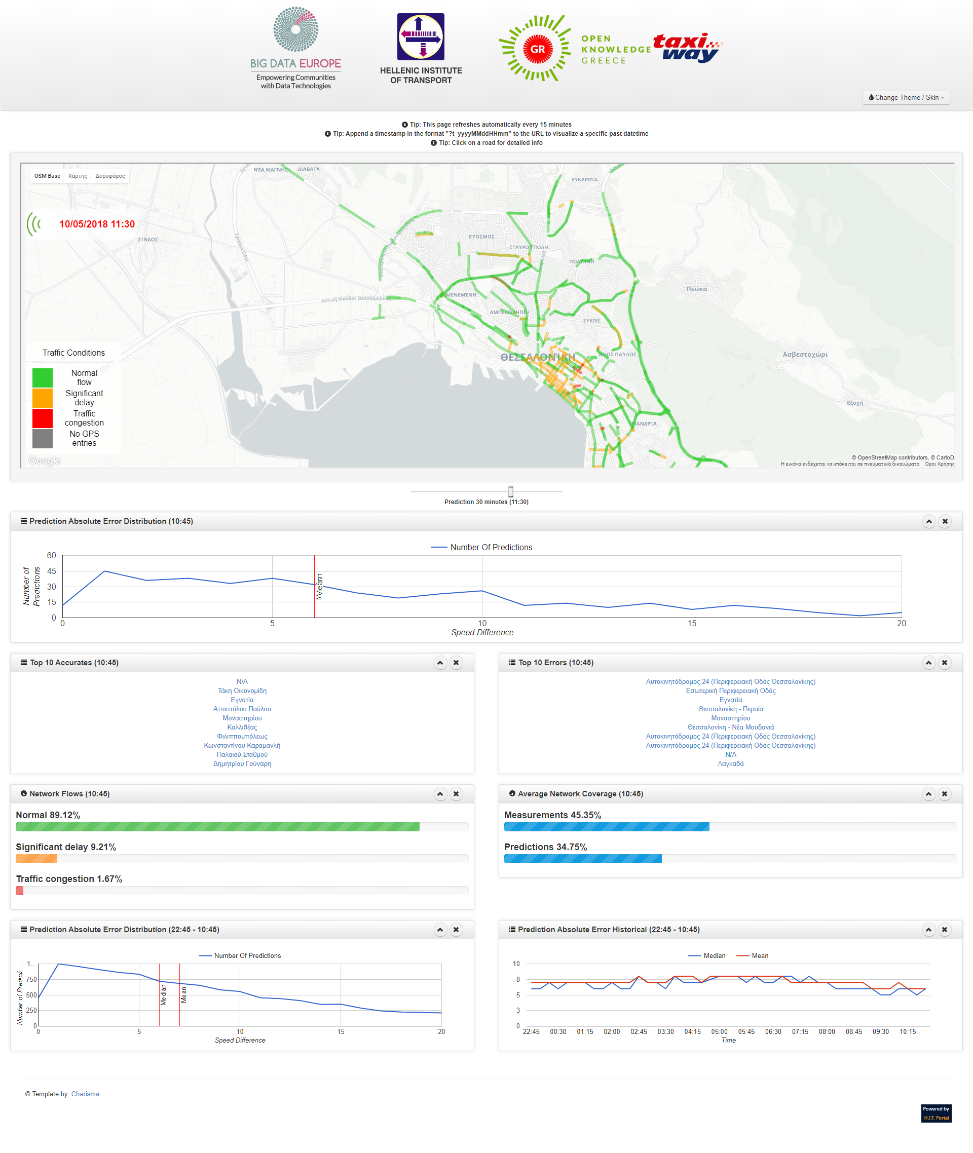
Traffic status prediction & statistics in real time
HIT partipiacted in TRANFOR19, a transportation forecasting competition organized by ABJ70 Artificial Intelligence and Advanced Computing Applications and supported by IEEE ITSS Technical Activities Sub-Committee “Smart Cities and Smart Mobility”
The scope of the competition is to evaluate the accuracy of statistical, or CI methods in transportation data forecasting with particular reference to short term traffic forecasting. The focus will be on obtaining predictions, as close as possible to the real data. Solutions that will advance the current understanding in advanced computing, data preprocessing and traffic dynamics will be also favored. The competition is open to Teams (single participant or group of participants) that are willing to present their work at the 2019 TRB Annual Meeting.
The available data sets include data for October and November of 2016 (61 text files in total). Each file contains information about the vehicle’s exact position on the road segment, the precise generation timestamp of the GPS entry, the driver and the order IDs. All IDs were encrypted and anonymized. Due to the large size and complexity of the input data sets, the first step on the data preparation stage was to import the text files into an RDBMS in order to perform basic data filtering and data transformations and to enable further processing. The RDBMS of our choice was the Microsoft SQL Server 2016 database software. During the data import phase, we performed the following actions on the complete data set:
• Creation of UTC+8 timestamp (local time in China) from the supplied epoch timestamp.
• Conversion of the GPS coordinates from the GCJ-02 to the WGS-84 projection system.
• Calculation of the distance travelled between subsequent GPS entries of the same driver and order (in meters).
• Estimation of the moving speeds (in km/hour) and orientations (in degrees from North).
• Whether a GPS entry was recorded inside the road section of interest (North or South) or not.
The import process took several hours to complete. The resulting table contained 1,560,295,942 rows and included the complete data from all 61 input files.
We continued the data preparation process by creating the appropriate database indexes in order to speed up the execution time of the queries we were to perform next. Then we calculated the following metrics in a five minutes time window: The minimum, maximum, average, median, interquartile mean, standard deviation, variation, skewness, kurtosis values of the observed moving speeds of the vehicles, as well as the total number of GPS entries, the number of unique trips and the number of unique vehicles that produced the GPS entries.
The next steps of analysis where completed in Python. Two main datasets were selected from the database. The first contains all historical GPS pulses on the targeted road section and the second contains pulses on 13 surrounding roads, which were defined as polygons in QGIS software and imported into Python for filtering. The python scripts for connecting to the SQL database and fetching requested data are ‘surrounding road data.py’ and ‘target road data.py’. The purpose of extracting data from surrounding roads was to examine correlation between average speeds of those roads and the targeted one. Since the volume of data was huge, surrounding road data were selected for only 8 days, from 14 to 18 and from 28 to 30 of November. Those days were picked because they are weekdays and according to historical weather sites the weather conditions those days were similar with the target day (1st December). The data from the above database queries were saved in pickle format:
a) target_road_north.pkl (target road north direction data)
b) target_road_south.pkl (target road south direction data)
c) dataset_ 28to30.pkl (surrounding roads pulse data, 28 to 30 November)
d) dataset_14to18.pkl (surrounding roads pulse data, 14 to 18 November)
As a next step, data from surrounding roads (c and d) were used as input by the module ‘group.py’, which groups GPS records in 5-minute time intervals, extracting distribution statistics. The outputs are saved as pickle files ‘aggregated_dataset_14to18.pkl’ and ‘aggregated_dataset_28to30.pkl’.
Two modules were developed for exploring the datasets. In the first script, ‘data exploration.py’, all datasets are imported, certain transformations are applied to the data and several plots and statistic results are produced. Outputs include time series plots, additive decomposition plots, average speed density plots, lag plots, autocorrelation plots, correlation matrix. The second script, ‘cross-corelation.py’, examines the existence of cross correlation between the targeted road average speed and surrounding roads speed at same interval and up to 3 lags in the past. Outputs from both modules suggest that the time series to be predicted has a strong seasonal component, and there is no strong correlation between the target road and the surrounding ones.
Three predictive models were developed for the purpose of this competition. All machine learning models were evaluated on test sets that were excluded from the training phase, and the hyper-parameter values for each model were optimized using the grid search cross validation method. The described procedures are explained in the models’ scripts in further detail. The python scripts for creating the predictive models are in the ‘scripts’ subfolder of our team’s submission file.
The first is a time series forecasting model that utilizes seasonal indices. This statistical method was implemented because it provides with accurate predictions on seasonal time series without trend, characteristics that were identified in the target time series. The whole procedure is explained and completed in python scripts ‘seas_ind_north.py’ and ‘seas_ind_south.py’, for north and south directions respectively. Each script outputs an excel file with predictions for a whole day, and values for the missing time periods were manually added in our team’s final predictions file. The scripts also produce visualization of results. This model’s strength is that it is highly accurate, easy to interpret, computationally inexpensive and therefore fast to implement. On the other hand, this method only works for seasonal time series without trend, so it would not be possible to use this method for predicting speed at other roads that do not have these characteristics.
The second model utilizes a state-of-the-art artificial neural network, a RNN with one hidden LSTM layer, specifically designed for time-series prediction. The model is trained with data from a 10-hour time window for one direction, with the first 5 hours used as model input and the other 5 hours as model output (target variable). Four python modules were developed, one for each direction and prediction time interval. Each module outputs two files, the first being the model saved in a format ready to be imported again to python for further analysis, and the second an excel file with the predictions for the corresponding 5-hour interval. The predictions are then manually added to the final prediction csv files.
LSTM models are known for their ability to learn long-term dependencies ‘hidden’ in time series. One disadvantage of utilizing LSTM in this competition is the relatively short duration of available timeseries data.
The third and final model approaches the problem with the same fashion as the LSTM model, utilizing consecutive 10-hour intervals for training, with 5-hour data as input and 5-hour data as target. Again, although the neural network has the capability of modeling complex relations amongst input and output data, the limited timespan of the timeseries is possible to limit the model’s ability for accurate predictions. Four dense neural network modules were also created for all direction and time-interval period combinations, and each of them outputs the neural network model and a file with the predicted average speeds, which are then manually added to the final prediction csv files. Both the dense and the LSTM neural networks have a significant advantage in the sense that they can be generalized and expanded to include more input features (variables) in order to enhance predictive accuracy. This is a powerful feature that would empower a real-world application for real-time traffic prediction. Our team developed a dense neural network utilizing data from surrounding roads, but the model’s predictive performance was poor, as predictions were conducted in a stepwise manner using recorded data from surrounding roads but also the predicted speed for the target road at previous steps.